Visualize hidden Markov model results — create_hmm

Generates a series of plots to visualize state assignments and the distribution of the surveillance signal across different hidden states.

Usage

create_hmm_plots(list_results, print = FALSE)

Arguments

list_results: An object of class epiquest_hmm produced by run_hmm().
print: A logical. If TRUE, all generated plots are printed to the active graphics device.

Value

An object of class epiquest_plot_list, a named list of ggplot2 objects containing:

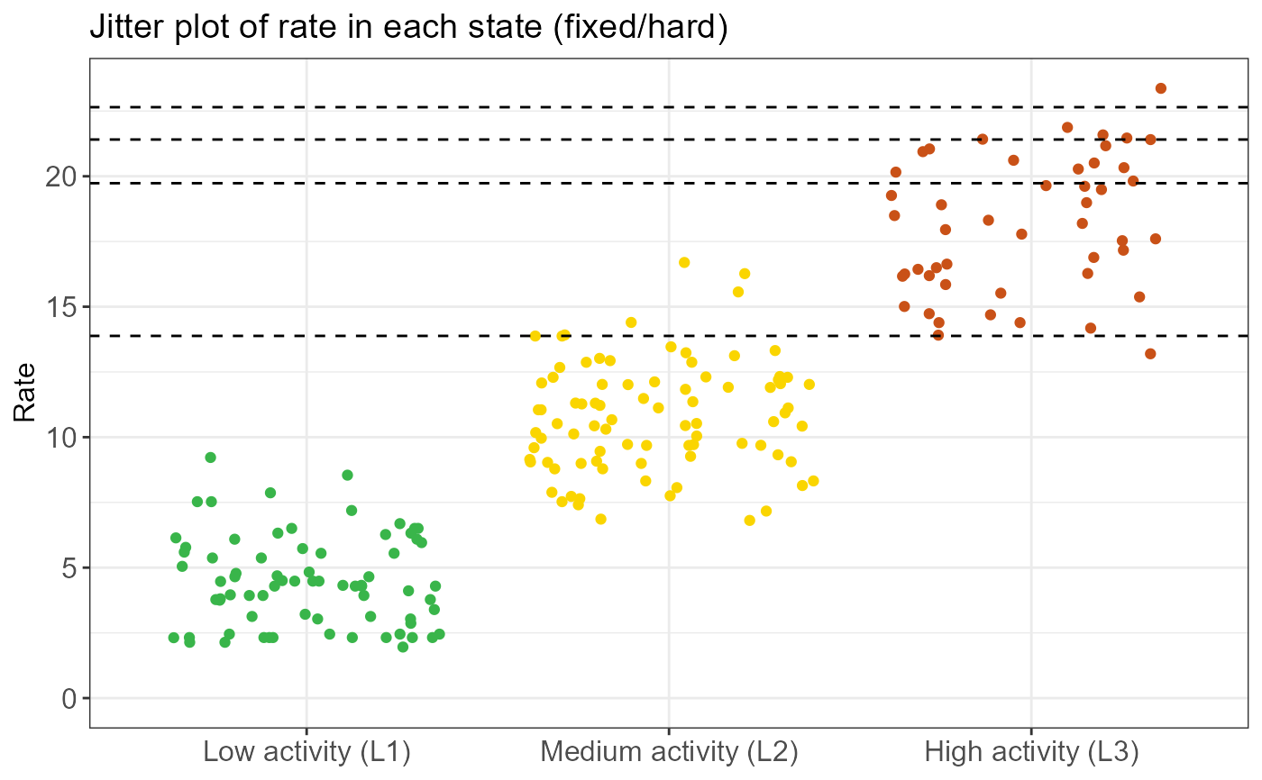
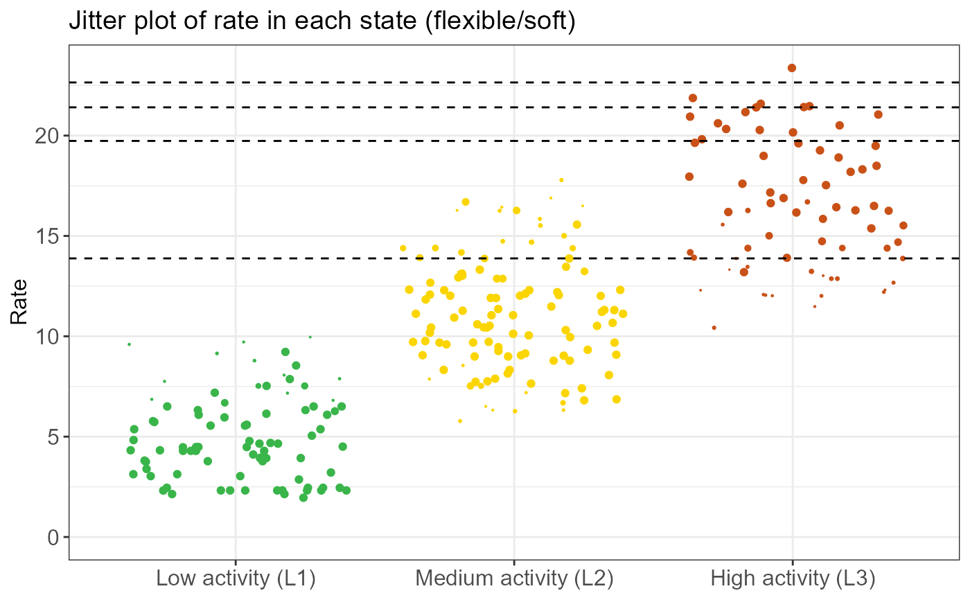
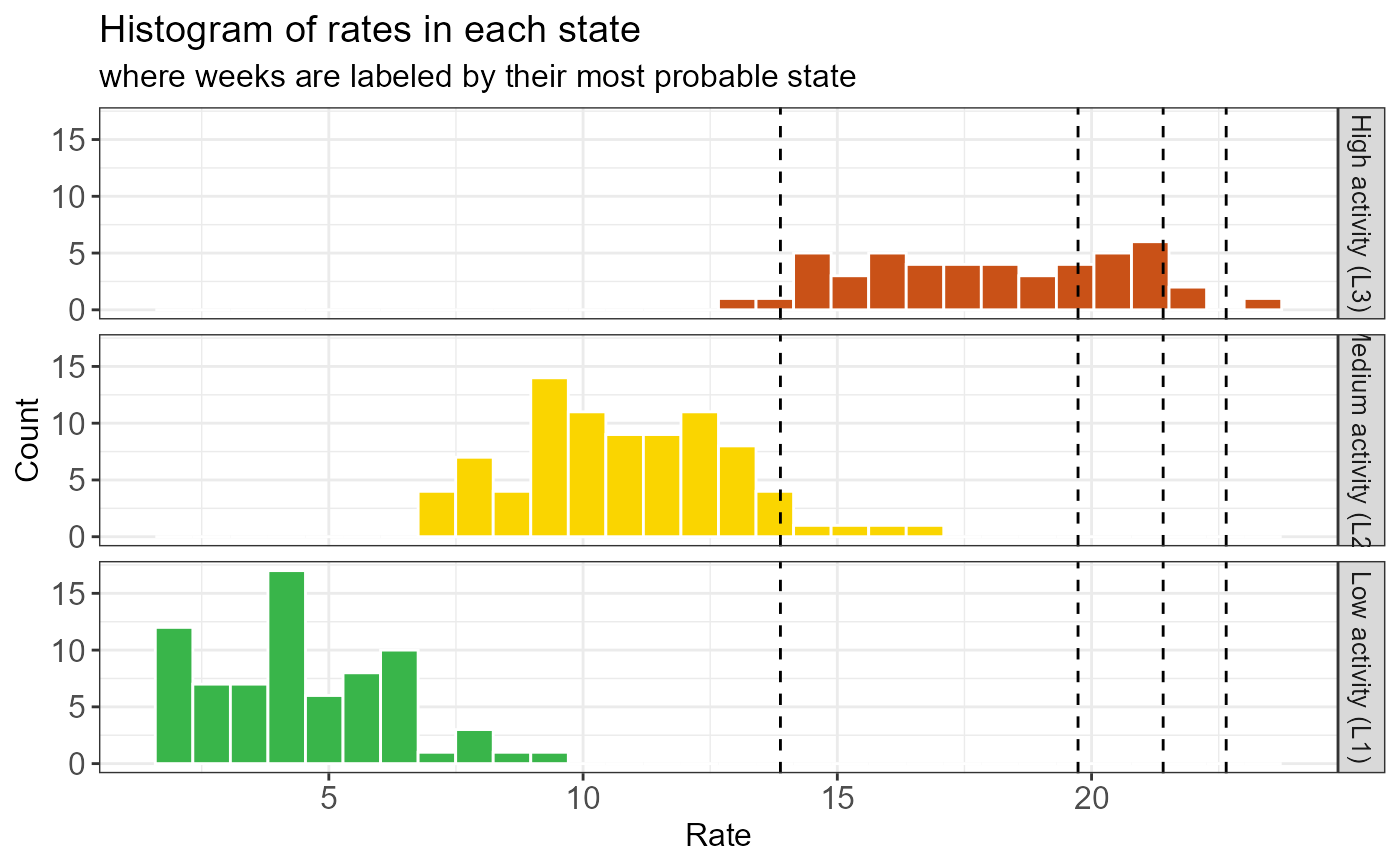
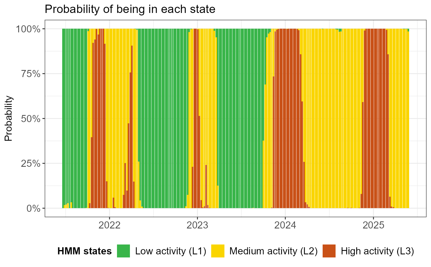
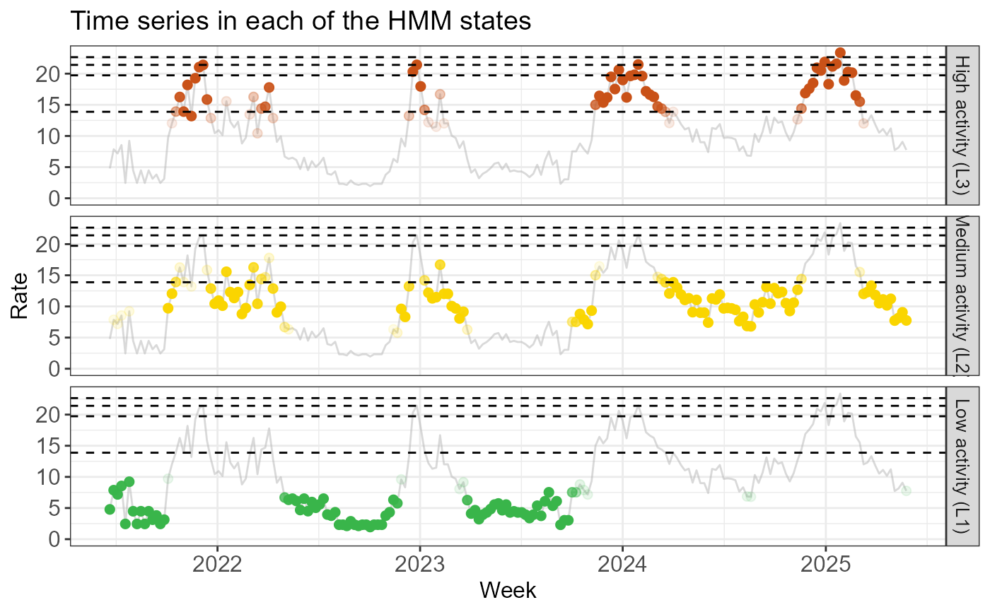
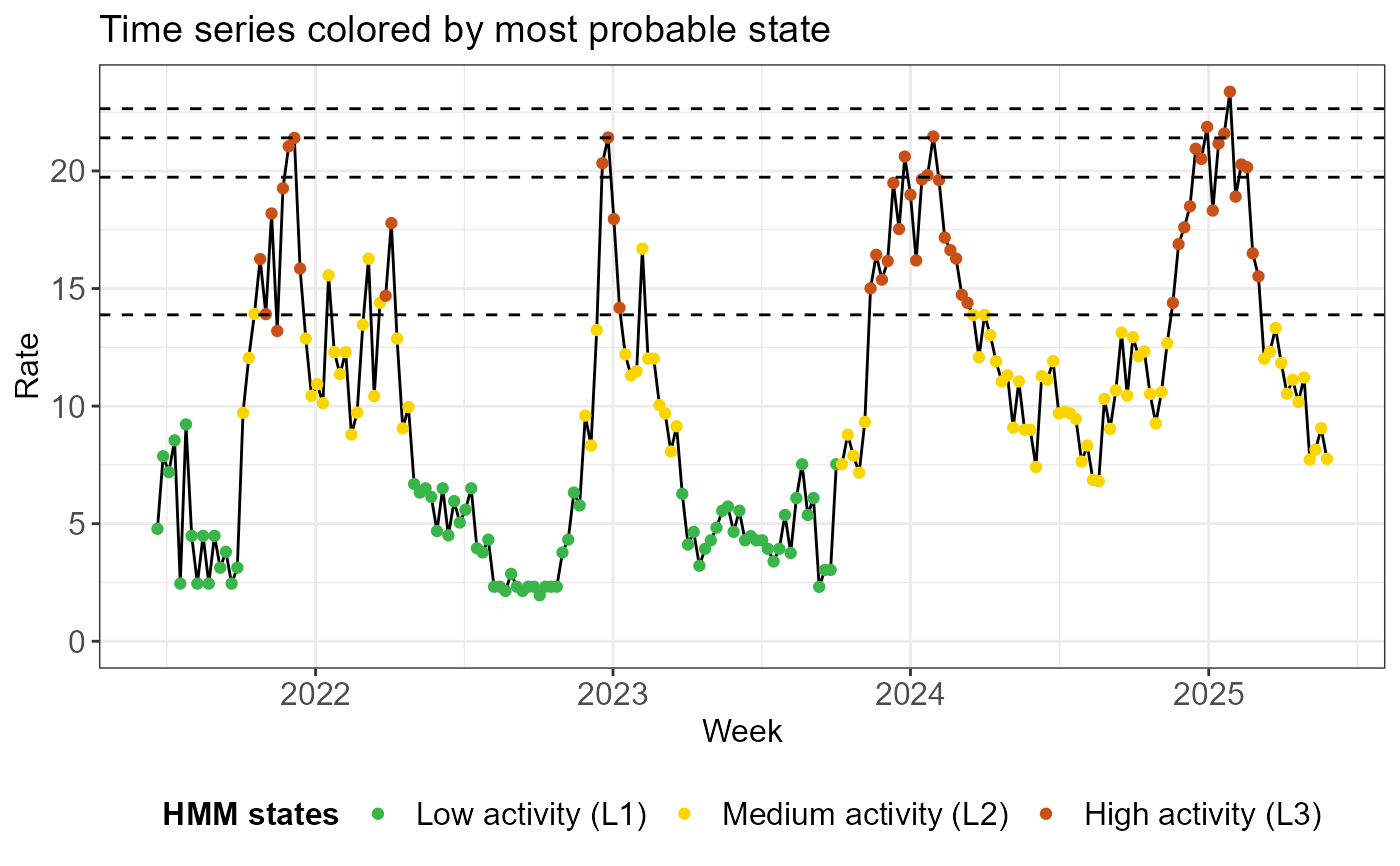
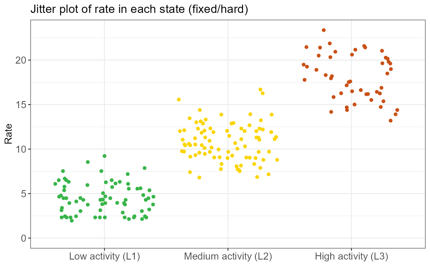
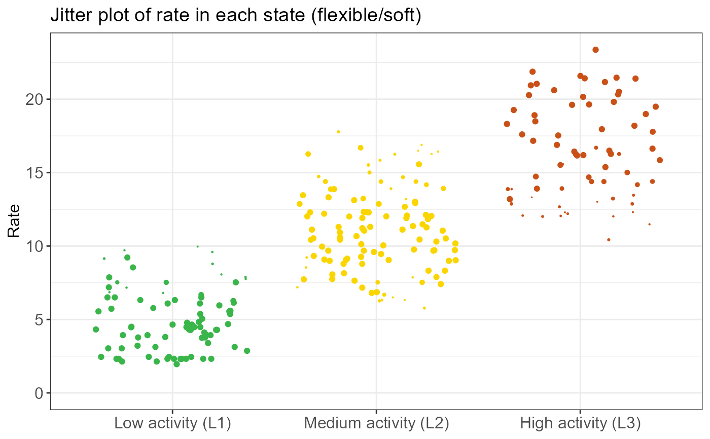
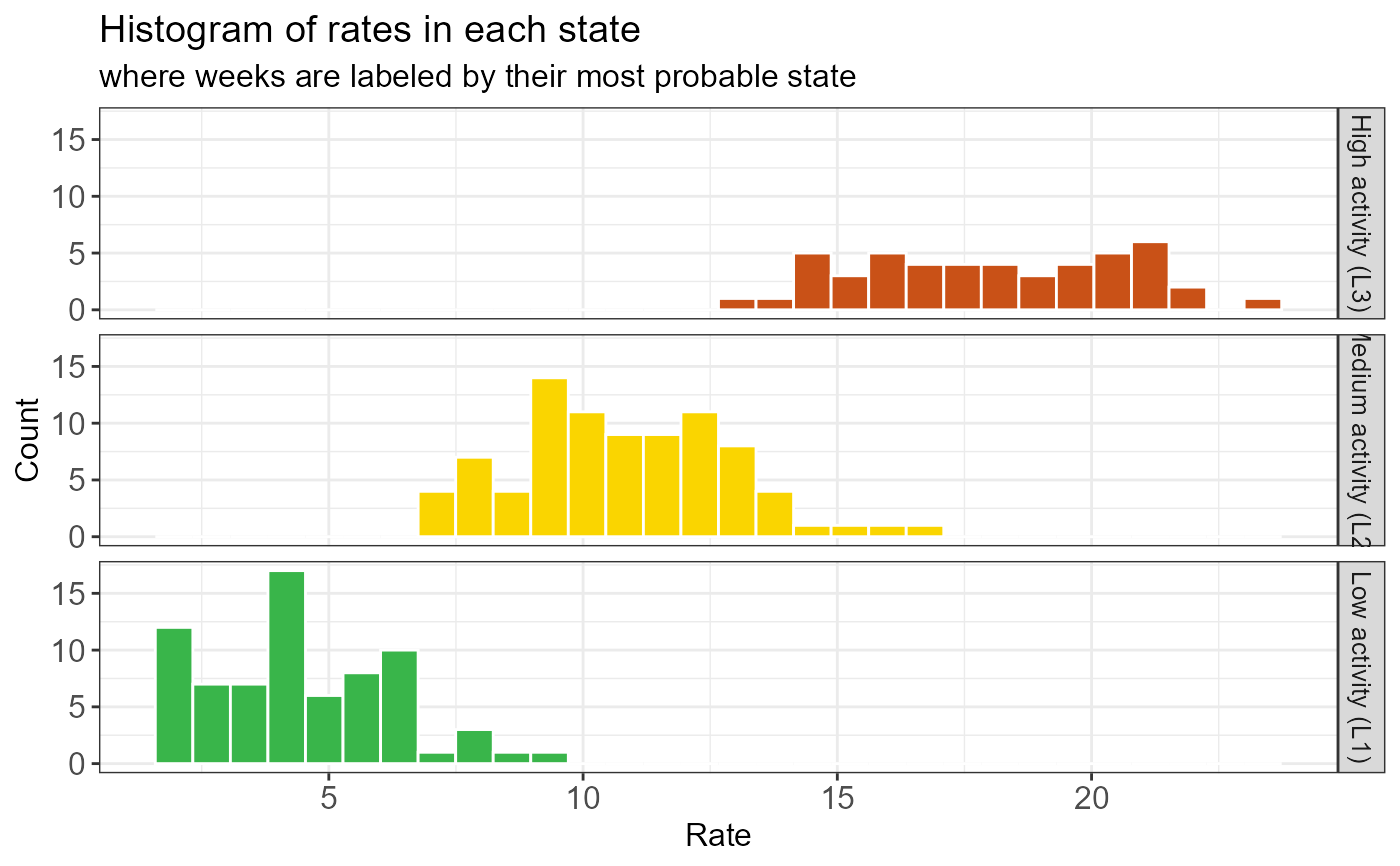
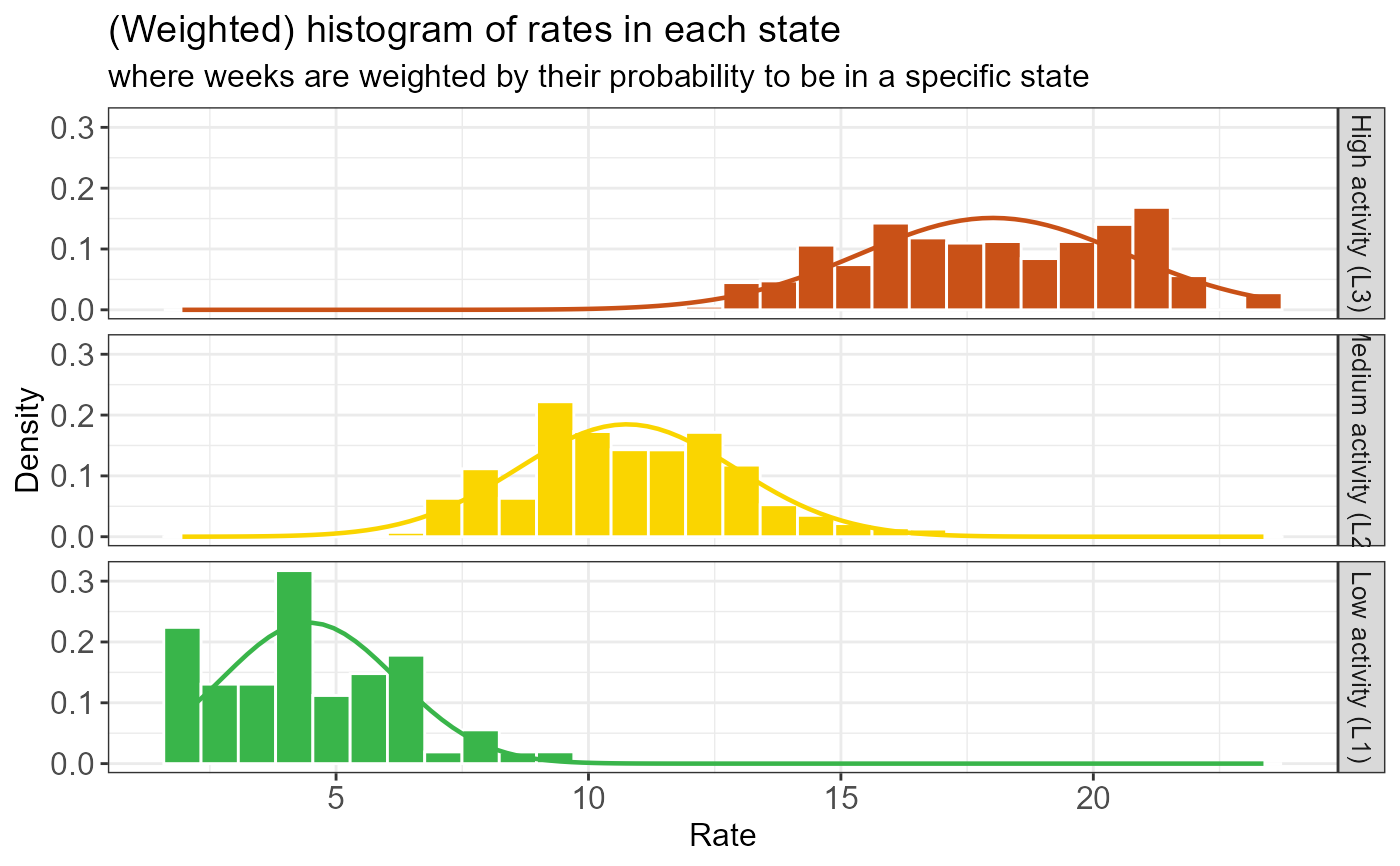
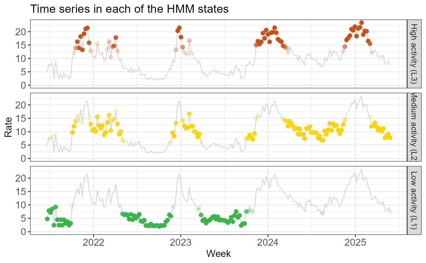
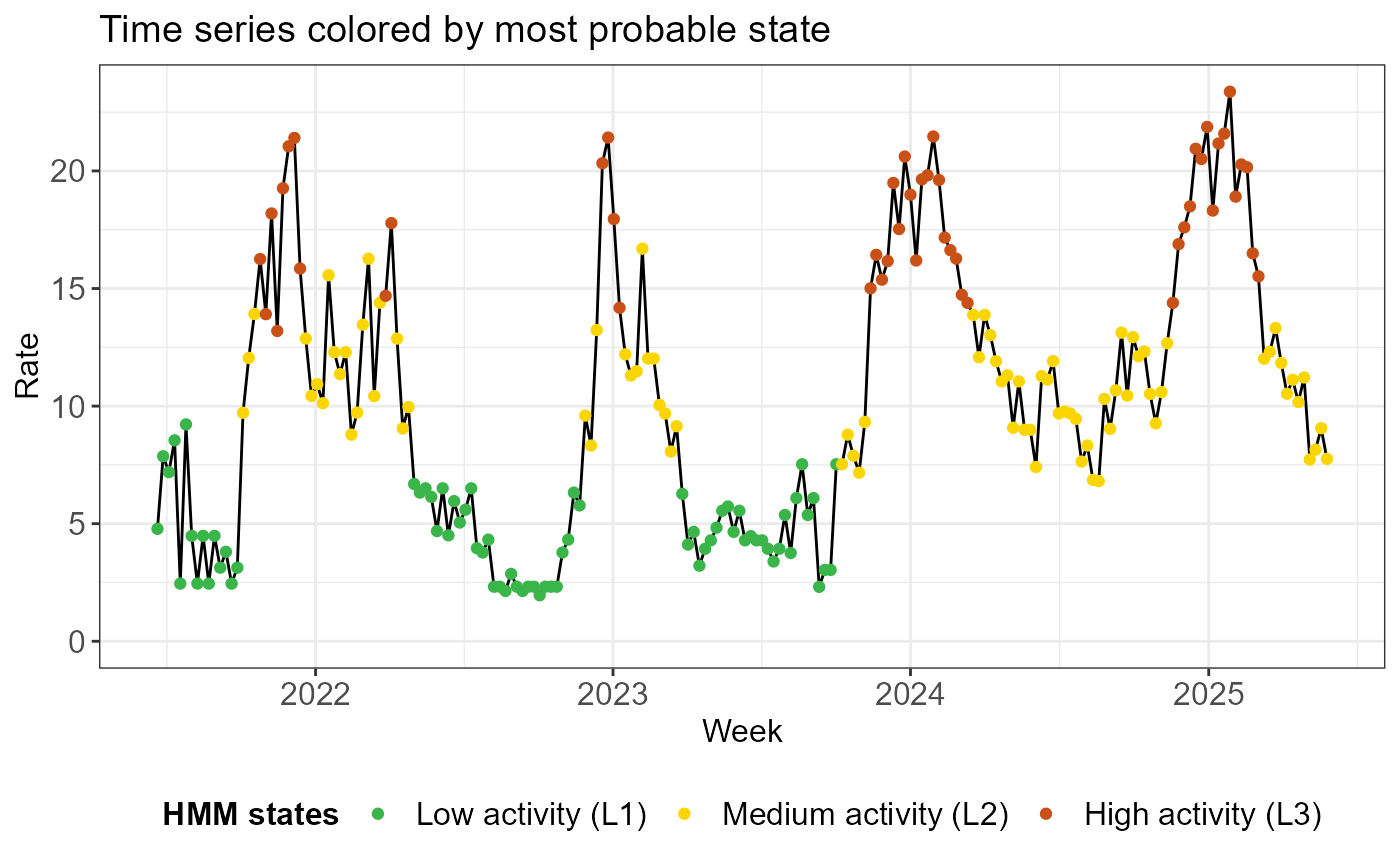
jitter_hard/soft Jitter plot showing signal distribution per state.
histogram_hard/soft Histogram showing signal density per state.
prob_states Stacked bar chart of posterior state probabilities.
time_series_per_state Faceted time series by state.
time_series_full Single time series colored by most probable state.

Details

The function produces several types of visualizations:

Time series: The raw signal colored by the most probable state.
Jitter plots and histograms: Visualize the overlap and separation between states.
State probabilities: A stacked bar chart showing the certainty of state assignments over time.

For many plots, both "hard" and "soft" versions are provided. Hard assignments classify a time point strictly into the single state with the highest posterior probability. Soft assignments weight each observation by its probability of belonging to each state, providing a more nuanced view of uncertainty.

Note

If list_results$type == "rate", the histogram_soft plot overlays the estimated Gaussian density curves for each state.

Examples

# Fit a 3-state HMM to (continuous) rate data
fit <- run_hmm(df_sari_be, n_states = 3, type = "rate")

# Check state information
summary(fit)
#> 
#> ========================================================
#>          EpiQUEST hidden Markov model summary           
#> ========================================================
#> 
#> --- Model configuration --------------------------------
#> Type:                    Continuous (Gaussian) 
#> Number of states:        3 
#> Seasonal:                FALSE 
#> Number of observations:  206 
#> 
#> --- Estimated state parameters -------------------------
#>  State   Mean Standard deviation
#>     L1  4.468              1.722
#>     L2 10.758              2.159
#>     L3 18.011              2.641
#> 
#> --- Transition matrix ----------------------------------
#>   State   ToL1   ToL2   ToL3
#>  FromL1 95.73%  4.27%  0.00%
#>  FromL2  2.51% 91.01%  6.48%
#>  FromL3  0.00% 11.32% 88.68%
#> 
#> --- State distribution (observations) ------------------
#>  State Total weight Proportion
#>     L1         72.6      35.2%
#>     L2         85.2      41.4%
#>     L3         48.2      23.4%
#> 
#> Note: Weights are posterior probabilities.
#> ========================================================

# Visualize state information
create_hmm_plots(fit)








# Compute thresholds using the highest state (L3) as the epidemic state
# By default, epidemic_state_indices is the highest state
thresh <- run_threshold_computation(fit)

# Visualize theshold information
summary(thresh)
#> 
#> ==============================================================
#>         EpiQUEST threshold summary                            
#> ==============================================================
#> 
#> --- Model configuration --------------------------------------
#> Type:                          Continuous (Gaussian) 
#> Number of states:              3 
#> Seasonal:                      FALSE 
#> Number of observations:        206 
#> State(s) defined as epidemic:  L3 
#> 
#> --- Calculated QUEST thresholds ------------------------------
#>      Level Quantile  Value
#>        Low       5% 13.881
#>     Medium      70% 19.734
#>       High      90% 21.408
#>  Very high      99% 22.647
#> 
#> Note: Thresholds calculated using weighted ECDF
#> based on posterior probabilities of epidemic state(s).
#> ==============================================================

# Visualize theshold information
create_threshold_plots(thresh)