Visualize hidden Markov model and threshold results

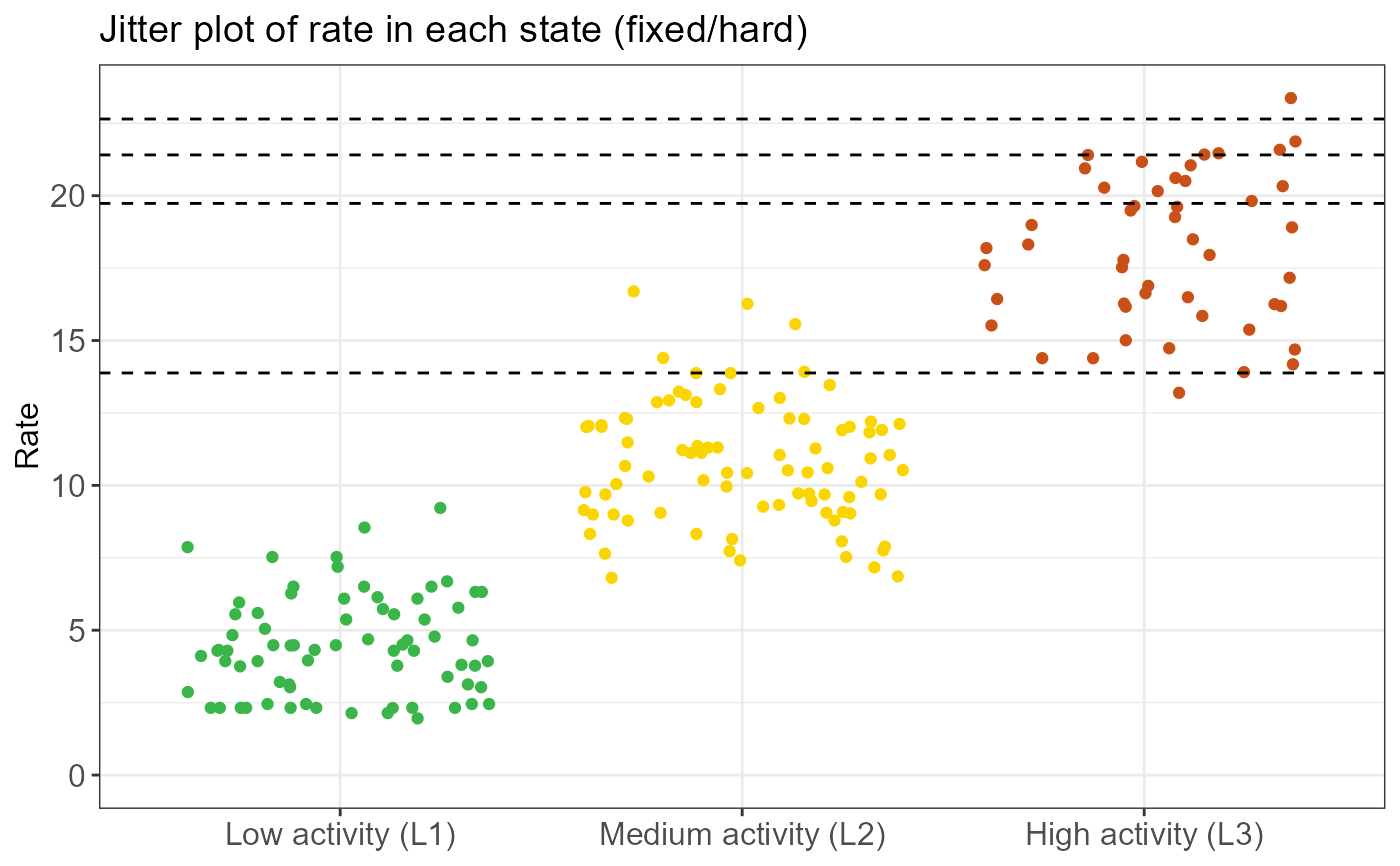
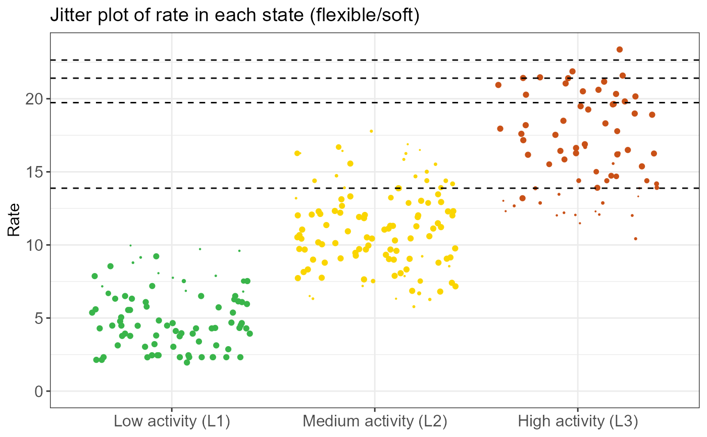
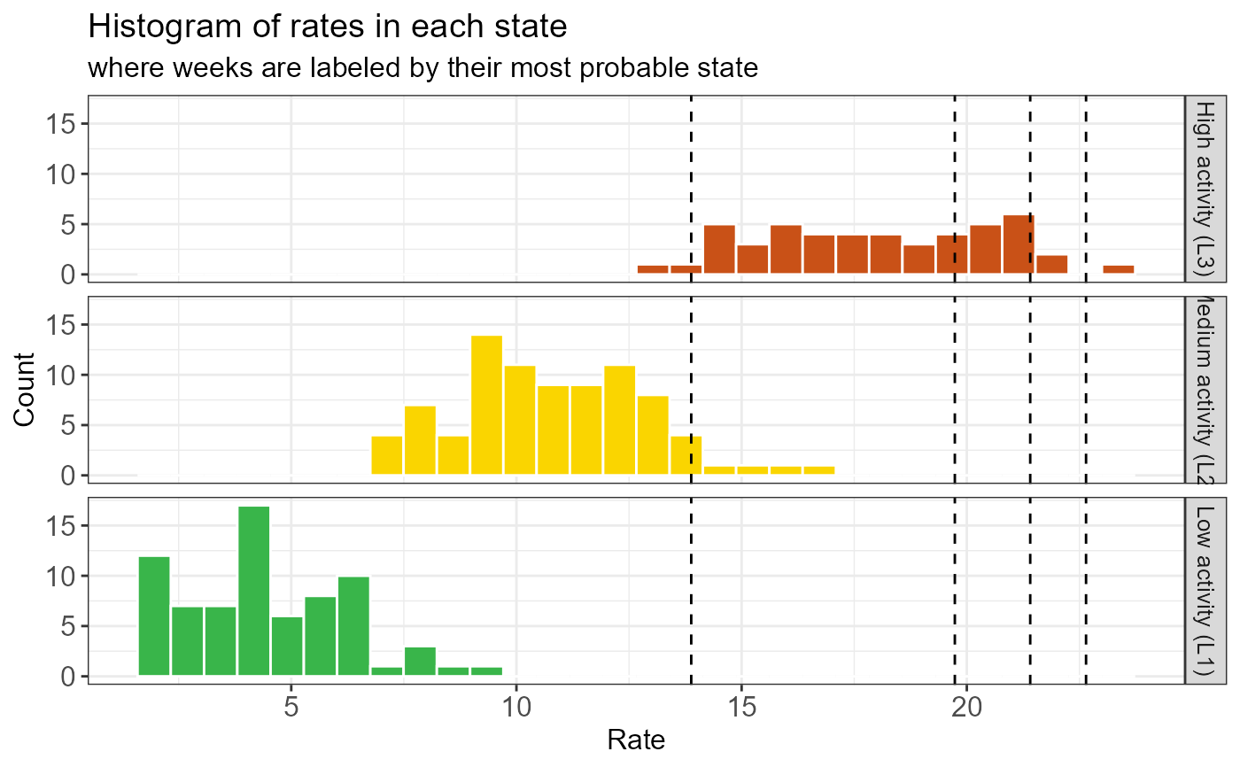
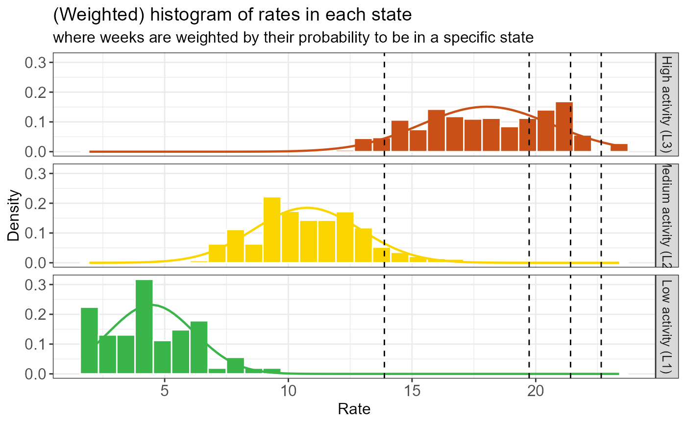
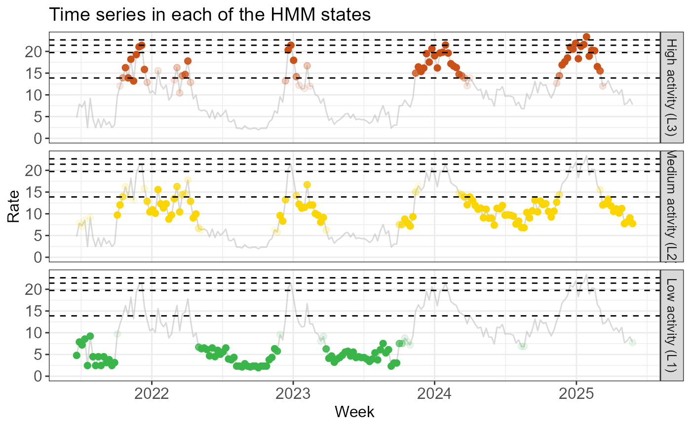
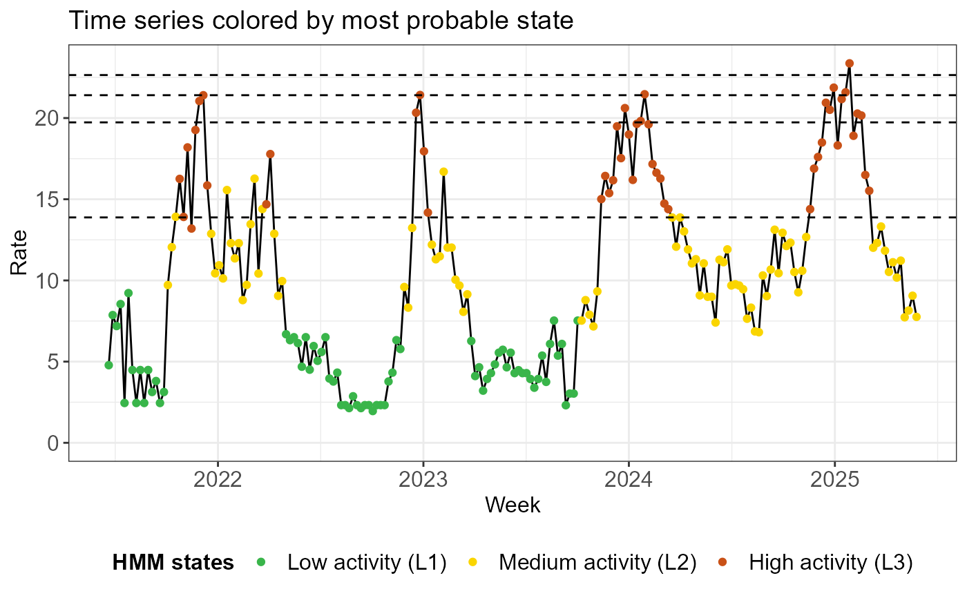
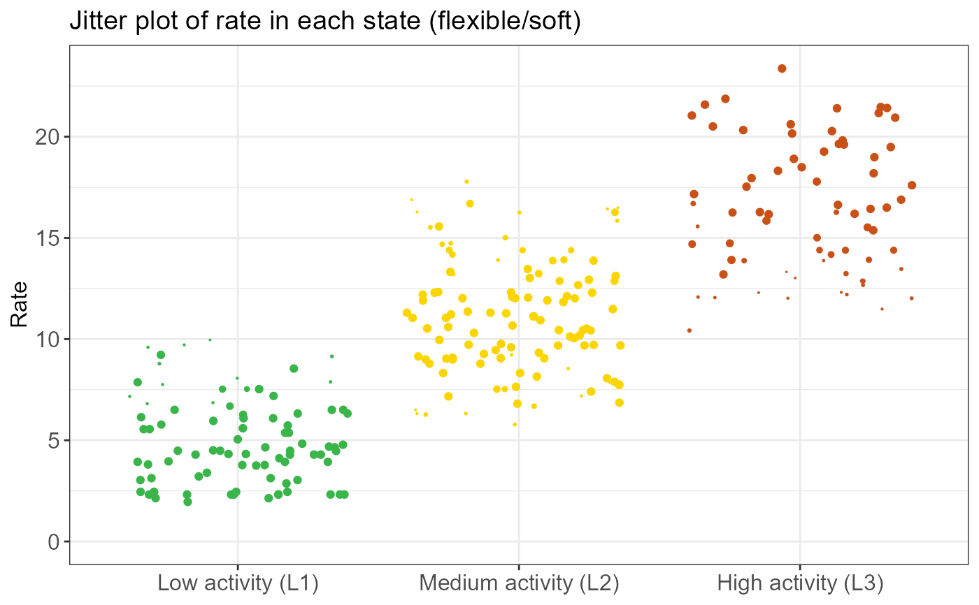
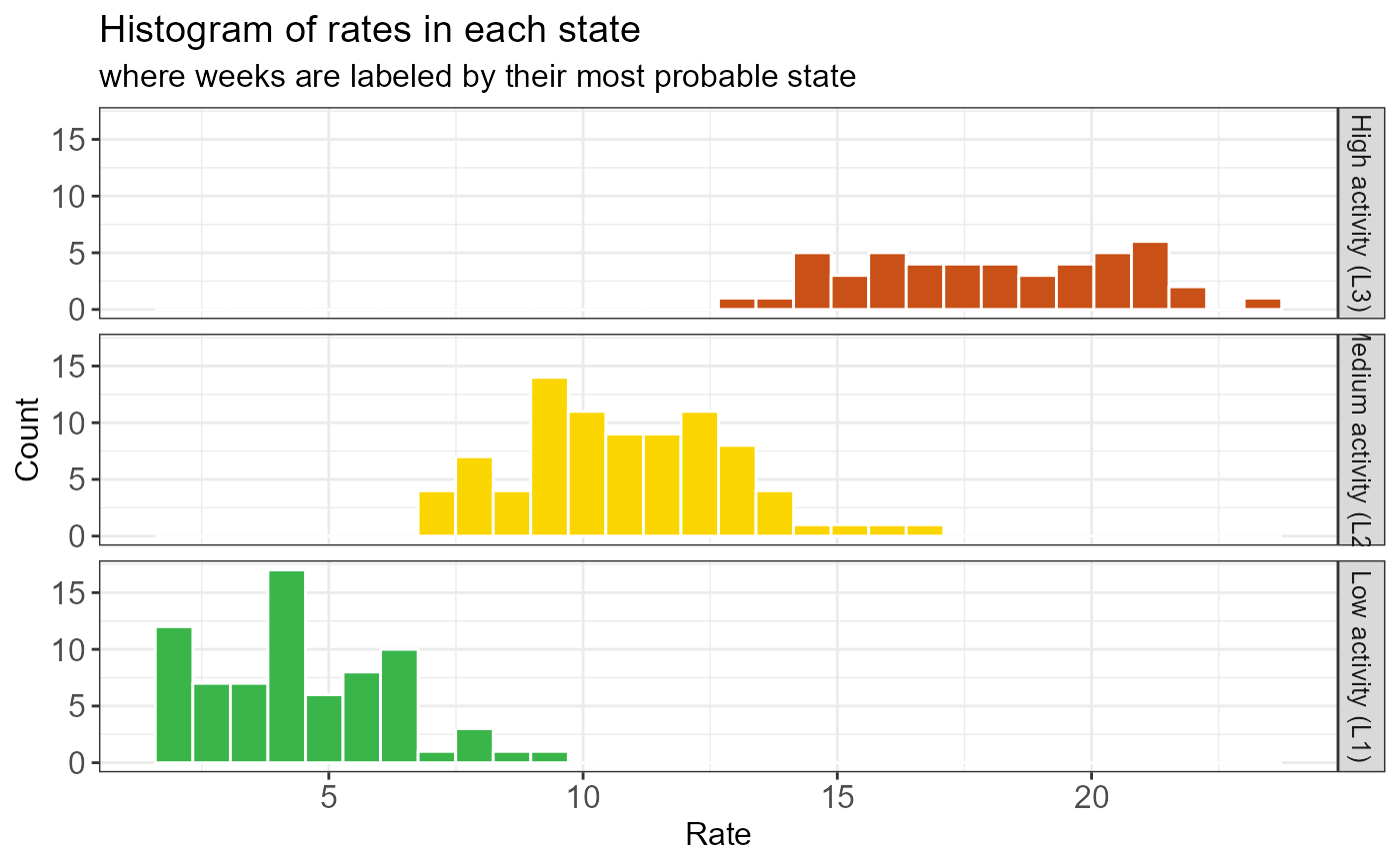
Extends the visualizations from create_hmm_plots() by adding horizontal or vertical dashed lines representing the calculated QUEST thresholds.

Usage

create_threshold_plots(list_results, print = FALSE)

Arguments

list_results

An object of class epiquest_thresholds produced by run_threshold_computation().

print

A logical. If TRUE, all generated plots are printed to the active graphics device.

Value

An object of class epiquest_plot_list, a named list of ggplot2 objects, identical in structure to the output of create_hmm_plots(), but with threshold lines added to:

• jitter_hard/soft

• histogram_hard/soft

• time_series_per_state

• time_series_full

Details

This function first calls create_hmm_plots() to generate the base visualizations. It then overlays dashed lines corresponding to the thresholds stored in the list_results object.

See also

run_threshold_computation, create_hmm_plots

Examples

# Fit a 3-state HMM to (continuous) rate data
fit <- run_hmm(df_sari_be, n_states = 3, type = "rate")

# Check state information
summary(fit)
#> 
#> ========================================================
#>          EpiQUEST hidden Markov model summary           
#> ========================================================
#> 
#> --- Model configuration --------------------------------
#> Type:                    Continuous (Gaussian) 
#> Number of states:        3 
#> Seasonal:                FALSE 
#> Number of observations:  206 
#> 
#> --- Estimated state parameters -------------------------
#>  State   Mean Standard deviation
#>     L1  4.468              1.722
#>     L2 10.758              2.159
#>     L3 18.011              2.641
#> 
#> --- Transition matrix ----------------------------------
#>   State   ToL1   ToL2   ToL3
#>  FromL1 95.73%  4.27%  0.00%
#>  FromL2  2.51% 91.01%  6.48%
#>  FromL3  0.00% 11.32% 88.68%
#> 
#> --- State distribution (observations) ------------------
#>  State Total weight Proportion
#>     L1         72.6      35.2%
#>     L2         85.2      41.4%
#>     L3         48.2      23.4%
#> 
#> Note: Weights are posterior probabilities.
#> ========================================================

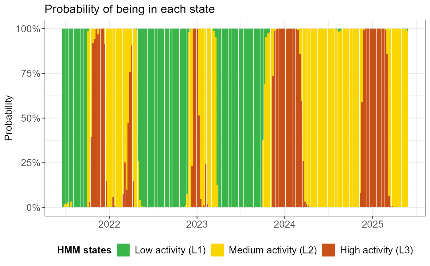
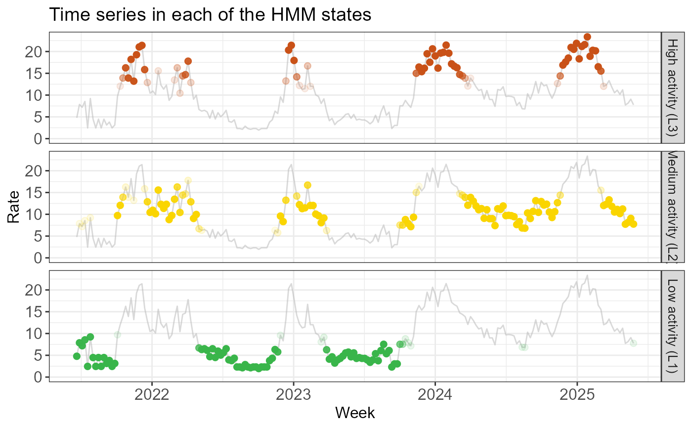
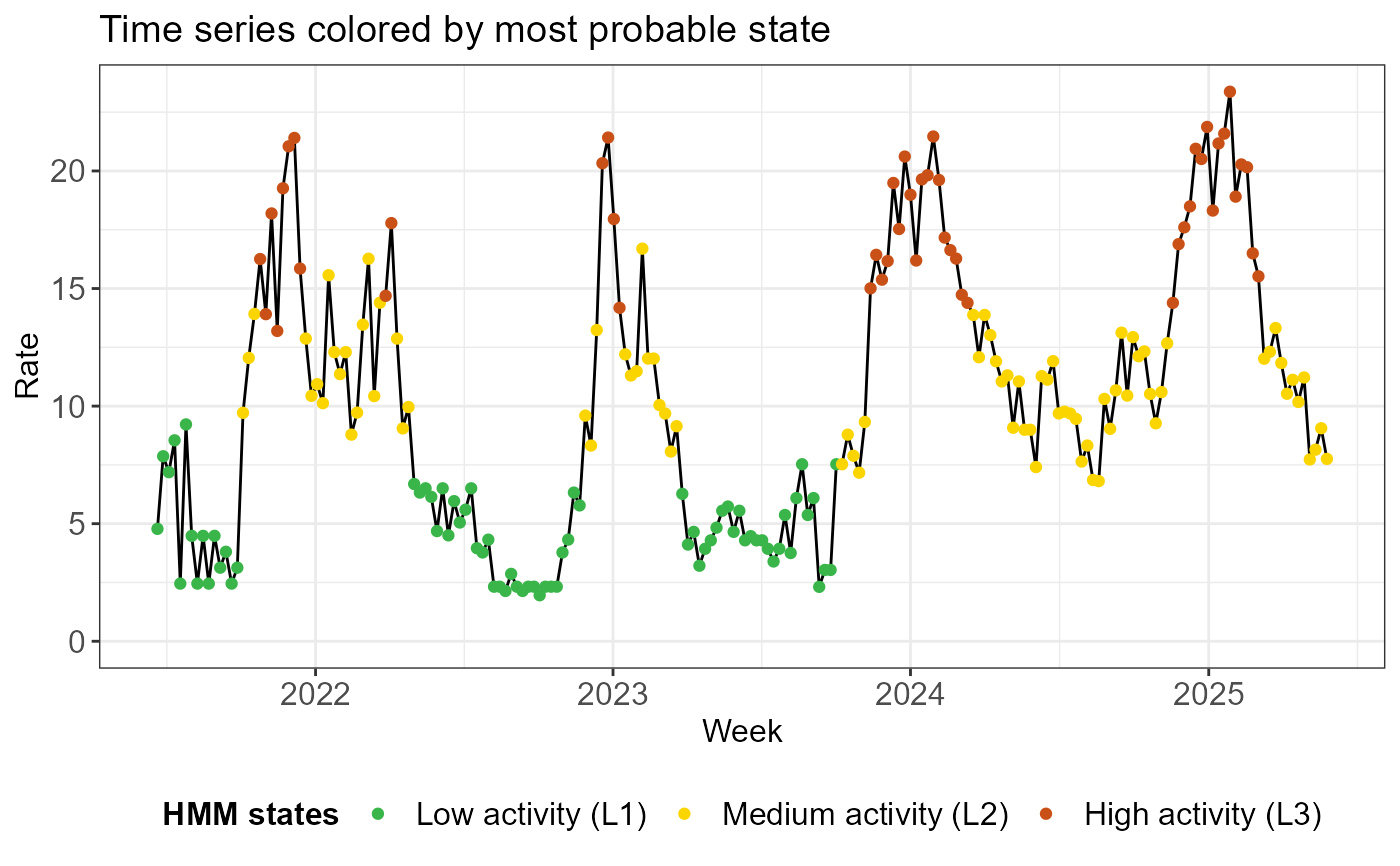
# Visualize state information
create_hmm_plots(fit)








# Compute thresholds using the highest state (L3) as the epidemic state
# By default, epidemic_state_indices is the highest state
thresh <- run_threshold_computation(fit)

# Visualize theshold information
summary(thresh)
#> 
#> ==============================================================
#>         EpiQUEST threshold summary                            
#> ==============================================================
#> 
#> --- Model configuration --------------------------------------
#> Type:                          Continuous (Gaussian) 
#> Number of states:              3 
#> Seasonal:                      FALSE 
#> Number of observations:        206 
#> State(s) defined as epidemic:  L3 
#> 
#> --- Calculated QUEST thresholds ------------------------------
#>      Level Quantile  Value
#>        Low       5% 13.881
#>     Medium      70% 19.734
#>       High      90% 21.408
#>  Very high      99% 22.647
#> 
#> Note: Thresholds calculated using weighted ECDF
#> based on posterior probabilities of epidemic state(s).
#> ==============================================================

# Visualize theshold information
create_threshold_plots(thresh)